Warning, if you plan to complete Advent of Code 2023, this post contains spoilers so don’t read it until you’re done.
My last post on Advent of Code spurred a bunch of discussion which inspired me to optimize my 2023 solutions in python even further. Where we left off: I had managed to get all my solutions running in under a second parallelized across multiple cores in python, and as a bonus had run all days solutions in parallel (again, multi-core) in about 1 second precisely. With the optimizations I’ll mention here, I’ve managed to get each solution working single-threaded in well under a second and all days running in parallel in under half a second on my 2021 M1 MacBook Pro.
| original runtime (s) | prev runtime (s) | new runtime (s) | Problem | Notes |
|---|---|---|---|---|
| 16.810 | 0.819 | 0.4452s | day23 | Using remapped graph, search from start to end and end to start, terminating at MID_DEPTH, join the paths. Believe a DP solution is possible. |
| 0.940 | 0.297 | 0.3478s | day16 | Don’t fire beam in on cells where a beam already exited |
| 2.412 | 0.376 | 0.2360s | day22 | Better algorithm - supports/supported_by vs dropping all bricks for pt2 |
| 1.057 | 0.471 | 0.2045s | day17 | thx azzal07, adapted bucket queue with 1D grid and unrolled neighbors inside dijkstra |
| 0.514 | 0.334 | 0.1805s | day14 | Use 1D grid coords and removed the rotate_clock fn which made a copy of the grid in favor of hand coded north, south, east, west roll functions |
| 0.413 | 0.281 | 0.1542s | day12 | thx rrutkows. Switched to an iterative soln vs DP |
| 8.463 | 0.108 | 0.1138s | day21 | garden |
| 0.188 | 0.107 | 0.1025s | day20 | digital logic and loops, seems optimized |
| 0.300 | 0.132 | 0.0990s | day25 | kargers (note: probabilistic, runtime varies) |
| 0.088 | 0.082 | 0.0823s | day07 | |
| 1.110 | 0.252 | 0.0625s | day24 | Reimplemented a purely algebraic solution |
| 0.076 | 0.064 | 0.0368s | day09 | |
| 0.062 | 0.061 | 0.0333s | day10 | Switched to shoelace and pick’s for pt2 |
| 0.073 | 0.042 | 0.0318s | day11 | |
| 0.047 | 0.046 | 0.0259s | day13 | |
| 0.048 | 0.048 | 0.0246s | day15 | |
| 0.126 | 0.044 | 0.0231s | day01 | |
| 0.211 | 0.030 | 0.0195s | day03 | |
| 0.040 | 0.039 | 0.0164s | day02 | |
| 0.037 | 0.037 | 0.0127s | day05 | |
| 0.035 | 0.034 | 0.0101s | day04 | |
| 0.041 | 0.041 | 0.0076s | day08 | |
| 0.065 | 0.045 | 0.0061s | day19 | |
| 0.040 | 0.033 | 0.0028s | day18 | |
| 0.140 | 0.032 | 0.0002s | day06 |
Here are a few additional lessons learned:
An algebraic solution to day 24
I initially solved part 2 of day 24: Never Tell Me The Odds, which amounted to a simultaneous equation of nine variables in nine unknowns, using sympy. Then replaced that with z3 which was faster. These are impressive tools which bundle up a plethora of mathematical methods to solve ~any system of equations you throw at them. During the live puzzle, I tried to solve part 2 algebraically with pen and paper, but gave up and moved to the library approach as my algebra is rather rusty! An algebraic solution should have a much faster runtime, so I was determined to find one. I saw a few comments on the subreddit suggesting it should be possible, so gave it a crack.
The most obvious way to approach an algebraic solution to this problem is to note that the “magic” stone needs to be at the same position as each of the hailstones at some time. In theory, you only need to consider the first three hailstones.
In vector form - the starting position plus \( t_{n} \) times the velocity of each hailstone must match the starting position (which is what we’re trying to determine for this problem) of the magic stone plus the same time \( t_{n} \) multiplied by the velocity of the magic stone. Thinking about the first three hailstones, in vector form that gives us these equations:
\(p_{magic} + t_0 . v_{magic} = p_0 + t_0 . v_0 \)
\(p_{magic} + t_1 . v_{magic} = p_1 + t_1 . v_1 \)
\(p_{magic} + t_2 . v_{magic} = p_2 + t_2 . v_2 \)
We know all the \(p_n\) and \(v_n\) values from the input data. These three equations can be expanded to nine equations (one each for \(x, y, z\) co-ordinates). That gives nine equations in nine unknowns: \(px_{magic} , py_{magic}, pz_{magic}, vx_{magic}, vy_{magic}, vz_{magic}, t_0, t_1, t_2 \)
| ———————— Stone 0 ———————— | ———————— Stone 1 ———————— | ———————— Stone 2 ———————— |
|---|---|---|
| \(px_{magic} + t_0 . vx_{magic} = px_0 + t_0 . vx_0 \) | \(px_{magic} + t_1 . vx_{magic} = px_1 + t_1 . vx_1 \) | \(px_{magic} + t_2 . vx_{magic} = px_2 + t_2 . vx_2 \) |
| \(py_{magic} + t_0 . vy_{magic} = py_0 + t_0 . vy_0 \) | \(py_{magic} + t_1 . vy_{magic} = py_1 + t_1 . vy_1 \) | \(py_{magic} + t_2 . vy_{magic} = py_2 + t_2 . vy_2 \) |
| \(pz_{magic} + t_0 . vz_{magic} = pz_0 + t_0 . vz_0 \) | \(pz_{magic} + t_1 . vz_{magic} = pz_1 + t_1 . vz_1 \) | \(pz_{magic} + t_2 . vz_{magic} = pz_2 + t_2 . vz_2 \) |
But, if you try to rearrange these you’ll find that this is not a linear system of equations (i.e. \(px\) also depends on \(vx\) etc). The trick is to figure out how to use what we know to find a linear system we can solve.
I tried plugging all of this into both sympy and Mathematica, asking for a symbolic solution for \( sx, sy, sz \) [which is hypothetically possible], but neither of them complete in reasonable time – in fact sympy eventually exhausted all the RAM on my machine (I think it’s the first time I’ve ever seen the “out of memory” dialog on Mac OS X Sonoma).

So is there a pen and paper solution? There’s perhaps a bit of a clue in the question, where we’re encouraged to ignore the z axis to get started. Initially, considering just the equations for x and y makes the system a bit easier to hold in your head and reason about.
Let’s also introduce some new terminology to make the math match the problem better: sx , sy and sz as the starting position of the magic stone, plus dx, dy, dz as its velocity and \(s_{00}\), \(s_{01}\), \(s_{02}\), \(s_{03}\), \(s_{04}\), \(s_{05}\) to represent the initial x,y,z position and dx,dy,dz velocity of hailstone 0 (similarly \(s_{10}\) is the x-coord of the starting position for hailstone 1 and \(s_{13}\) is dx for hailstone 1)
Now, we can re-write the first observation that the “magic” stone needs to be at the same position as each of the hailstones at some time for hailstone 0 in the x and y axes only as:
\(sx + t_0 dx = s_{00} + t_0 s_{03} \hskip{40px} \enclose{circle}{1} \)
\(sy + t_0 dy = s_{01} + t_0 s_{04} \hskip{40px} \enclose{circle}{2} \)
From (1), we can rearrange to find an equation for \( t_0 \)
\( t_0 (dx - s_{03}) = s_{00} - sx \)
\( t_0 = \frac{s_{00} - sx}{dx - s_{03}} \hskip{40px} \enclose{circle}{3} \)
\( t_0 (dy - s_{04}) = s_{01} - sy \)
\( t_0 = \frac{s_{01} - sy}{dy - s_{04}} \hskip{40px} \enclose{circle}{4} \)
Now setting \( \enclose{circle}{3} = \enclose{circle}{4} \)
\( \frac{s_{00} - sx}{dx - s_{03}} = \frac{s_{01} - sy}{dy - s_{04}} \)
Cross-multiply
\( (dy - s_{04})(s_{00} - sx) = (s_{01} - sy)(dx - s_{03}) \)
\( dy.s_{00} - dy.sx - s_{04} s_{00} + s_{04}.sx = s_{01}.dx - s_{01} s_{03} - sy.dx + sy.s_{03} \)
Rearrange to give us:
\( dy.s_{00} - dy.sx - s_{04} s_{00} + s_{04}.sx - s_{01}.dx + s_{01} s_{03} + sy.dx - sy.s_{03} = 0 \hskip{40px} \enclose{circle}{5} \)
With the same steps, we can find the same equation for the second hailstone (note how the \( s_{xx} \) terminology makes this easy to see ):
\( dy.s_{10} - dy.sx - s_{14} s_{10} + s_{14}.sx - s_{11}.dx + s_{11} s_{13} + sy.dx - sy.s_{13} = 0 \hskip{40px} \enclose{circle}{6} \)
Now here’s the cool part - if we find \( \enclose{circle}{5} - \enclose{circle}{6} \) the non-linear \( dy.sx, dx.sy\) terms cancel:
\( dy.s_{00} - s_{04}.s_{00} + s_{04}.sx - s_{01}.dx + s_{01}.s_{03} - sy.s_{03} - dy.s_{10} + s_{14}.s_{10} - s_{14}.sx + s_{11}.dx - s_{11}.s_{13} + sy.s_{13} = 0 \)
Collecting the \( sx, sy, dx, dy \) factors we have:
\( \large{ (s_{04} - s_{14}).sx + (s_{13} - s_{03}).sy + (s_{11} - s_{01}).dx + (s_{00} - s_{10}).dy = s_{04}.s_{00} - s_{01}.s_{03} - s_{14}.s_{10} + s_{11}.s_{13} } \)
This is a linear equation in all the unknowns - all the \( s_{xx} \) terms are already known from our input data. We can generate as many of these as we need from any pair of hailstones in our input data. As we have four unknowns, we’ll need 4 pairs of stones.
\( \large{ (s_{04} - s_{14}).sx + (s_{13} - s_{03}).sy + (s_{11} - s_{01}).dx + (s_{00} - s_{10}).dy = s_{04}.s_{00} - s_{01}.s_{03} - s_{14}.s_{10} + s_{11}.s_{13} } \) \( \large{ (s_{14} - s_{24}).sx + (s_{23} - s_{13}).sy + (s_{21} - s_{11}).dx + (s_{10} - s_{20}).dy = s_{14}.s_{10} - s_{11}.s_{13} - s_{24}.s_{20} + s_{21}.s_{23} } \) \( \large{ (s_{24} - s_{34}).sx + (s_{33} - s_{23}).sy + (s_{31} - s_{21}).dx + (s_{20} - s_{30}).dy = s_{24}.s_{20} - s_{21}.s_{23} - s_{34}.s_{30} + s_{31}.s_{33} } \) \( \large{ (s_{34} - s_{44}).sx + (s_{43} - s_{33}).sy + (s_{41} - s_{31}).dx + (s_{30} - s_{40}).dy = s_{34}.s_{30} - s_{31}.s_{33} - s_{44}.s_{40} + s_{41}.s_{43} } \)
Here’s the same thing in matrix form:
\( \begin{bmatrix} s_{04} - s_{14} & s_{13} - s_{03} & s_{11} - s_{01} & s_{00} - s_{10} \\ s_{14} - s_{24} & s_{23} - s_{13} & s_{21} - s_{11} & s_{10} - s_{20} \\ s_{24} - s_{34} & s_{33} - s_{23} & s_{31} - s_{21} & s_{20} - s_{30} \\ s_{34} - s_{44} & s_{43} - s_{33} & s_{41} - s_{31} & s_{30} - s_{40} \end{bmatrix} \begin{bmatrix} sx \\ sy \\ dx \\ dy \end{bmatrix} = \begin{bmatrix} s_{04}.s_{00} - s_{01}.s_{03} - s_{14}.s_{10} + s_{11}.s_{13} \\ s_{14}.s_{10} - s_{11}.s_{13} - s_{24}.s_{20} + s_{21}.s_{23} \\ s_{24}.s_{20} - s_{21}.s_{23} - s_{34}.s_{30} + s_{31}.s_{33} \\ s_{34}.s_{30} - s_{31}.s_{33} - s_{44}.s_{40} + s_{41}.s_{43} \end{bmatrix} \)
These form a system of linear equations of the form \( Ax = b \) so we can use any linear algebra solver or standard methods like Gaussian elimination or Cramer’s rule to solve.
Now, a quick aside: terms like “linear algebra” and “Gaussian elimination” might sound daunting at first. However, they are concepts that are much more approachable than they initially appear - I learned about both of them in high school, without the fancy names. For a clearer understanding, I recommend checking out this really old Khan Academy video, which provides an excellent beginner level introduction to these topics.
We can compute every one of those terms from the input data:
s = list(map(ints, [i.strip() for i in open("input","r").readlines()]))

A = [[s[0][4] - s[1][4], s[1][3] - s[0][3], s[1][1] - s[0][1], s[0][0] - s[1][0]],
     [s[1][4] - s[2][4], s[2][3] - s[1][3], s[2][1] - s[1][1], s[1][0] - s[2][0]],
     [s[2][4] - s[3][4], s[3][3] - s[2][3], s[3][1] - s[2][1], s[2][0] - s[3][0]],
     [s[3][4] - s[4][4], s[4][3] - s[3][3], s[4][1] - s[3][1], s[3][0] - s[4][0]]]
b = [s[0][4] * s[0][0] - s[0][1] * s[0][3] - s[1][4] * s[1][0] + s[1][1] * s[1][3],
     s[1][4] * s[1][0] - s[1][1] * s[1][3] - s[2][4] * s[2][0] + s[2][1] * s[2][3],
     s[2][4] * s[2][0] - s[2][1] * s[2][3] - s[3][4] * s[3][0] + s[3][1] * s[3][3],
     s[3][4] * s[3][0] - s[3][1] * s[3][3] - s[4][4] * s[4][0] + s[4][1] * s[4][3]]
Remember, I’m in search of a faster solution to day23 than z3 so I tried some solver libraries first. numpy works but produces inexact answers, mpmath produces an exact answer and is a lot faster than the original z3 approach given we’ve done the hard stuff already.
import mpmath

x = mpmath.lu_solve(A, b)
Ultimately, though, having come so far I didn’t want to use a library at all, so wrote a gaussian elimination function.
# Solve using Gaussian Elimination
x = [round(i) for i in gaussian_elimination(Ab)]

sx, sy, dx, dy = x
This gives us sx and sy but the question wants the sum of those and sz - to complete the algebraic solution we need a formula for sz. Given what we already know, this is a much simpler case than the linear algebra above.
Recall \( \enclose{circle}{3} \) : \( t_0 = \frac{s_{00} - sx}{dx - s_{03}} \) and similarly \( t_1 = \frac{s_{10} - sx}{dy - s_{13}} \)
\( t_0 \) and \( t_1 \) are the times that hailstones 0 and 1 respectively collide with the magic stone and together with the input data give us the exact positions of each stone at those times. Since the magic stone has constant velocity we can use \( distance = velocity * time \) to arrive at a formula for sz.
\( dz = \frac{pz_{1}(t_{1}) - pz_{0}(t_{0})}{t_1 - t_0}\) – This is just the equation for velocity between positions given time elapsed.
Which is:
\( dz = ((s_{12} + t_{1}*s_{15}) - (s_{02} + t_{0}*s_{05})) / (t_{1} - t_0) \)
and we can work back to an equation for sz:
\( sz = -t_1 * dz + s_{12} + t_1 * s_{15} \)
The whole solution is now done and it’s just the following python code:
Ab = [[s[0][4] - s[1][4], s[1][3] - s[0][3], s[1][1] - s[0][1], s[0][0] - s[1][0], s[0][4] * s[0][0] - s[0][1] * s[0][3] - s[1][4] * s[1][0] + s[1][1] * s[1][3]],
      [s[1][4] - s[2][4], s[2][3] - s[1][3], s[2][1] - s[1][1], s[1][0] - s[2][0], s[1][4] * s[1][0] - s[1][1] * s[1][3] - s[2][4] * s[2][0] + s[2][1] * s[2][3]],
      [s[2][4] - s[3][4], s[3][3] - s[2][3], s[3][1] - s[2][1], s[2][0] - s[3][0], s[2][4] * s[2][0] - s[2][1] * s[2][3] - s[3][4] * s[3][0] + s[3][1] * s[3][3]],
      [s[3][4] - s[4][4], s[4][3] - s[3][3], s[4][1] - s[3][1], s[3][0] - s[4][0], s[3][4] * s[3][0] - s[3][1] * s[3][3] - s[4][4] * s[4][0] + s[4][1] * s[4][3]]]

# Solve using Gaussian Elimination
x = [round(i) for i in gaussian_elimination(Ab)]

sx, sy, dx, dy = x

# From above.
t0 = (s[0][0] - sx) / (dx - s[0][3])
t1 = (s[1][0] - sx) / (dx - s[1][3])

# This is just the equation for velocity between positions given time
# elapsed.
dz = ((s[1][2] + t1*s[1][5]) - (s[0][2] + t0*s[0][5])) / (t1 - t0)

# sz + t1 dz - s12 - t1 s15 = 0
# sz = -t1 dz +s12 + t1 s15
sz = -t1 * dz + s[1][2] + t1*s[1][5]

print(int(sx)+int(sy)+int(sz))
This, together with part 1 runs in 0.0625s - a pretty handy 18x improvement on my original solution, with no third party library dependency to boot!
Working this through really helped polish up my very rusty high school algebra and I’m quite looking forward to helping my kids grok simultaneous equations when that comes up on their school math curriculum!
Going in both directions for day 23
Day 23: A long walk requires an exhaustive search to find the longest possible path in a maze. I had only managed to get it running in sub-second time by sharding the work across cores. However, ZeCookiez suggested an even better algorithm here which I had fun implementing.
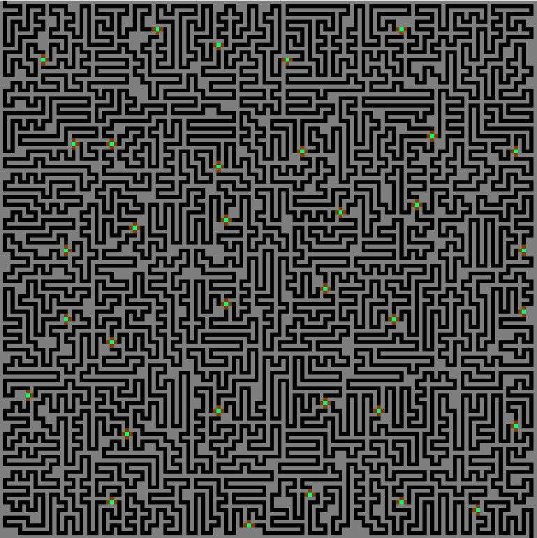
In this problem, we need to find the longest path from start to finish which doesn’t step on any square twice. Here’s what the maze looks like, with the start at the upper left and end at lower right. The green dots are spots in the maze where there are multiple directions you could go in vs being part of a long corridor.
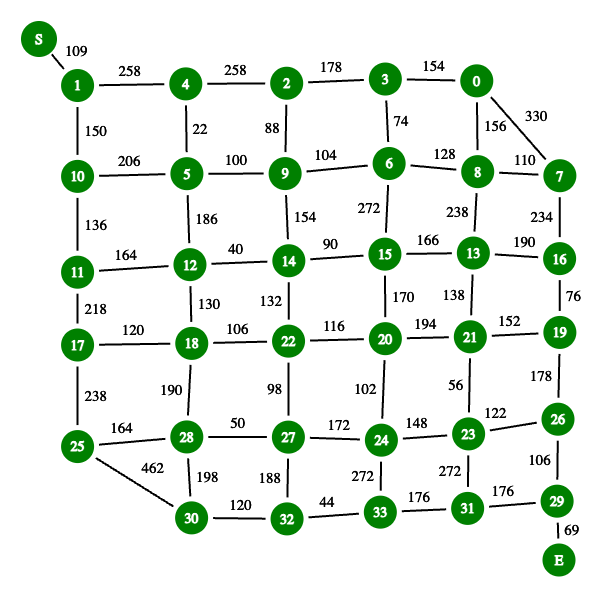
Noting that the maze mostly consists of relatively long twisting passageways and few intersections where we need to make choices about which route to take, I had already compressed the search space for this problem into the following graph, which I searched exhaustively, with some neat bitmasking to keep track of visited nodes quite quickly.
One immediate optimization you’ve probably spotted already is that the start and end edges (from S → 1 and 29 → E above) must always be followed, so we can just prune those from the search space, start at node 1 and end at node 29 and always add the mandatory path weights to the total.
But the real new trick is much cleverer - we can run the search from the start trying to get towards the end and again from the end trying to get back to any nodes we managed to get to from the start while capping the total depth of nodes visited in either direction at half of the total nodes in the graph (any non-overlapping longest path by definition can’t traverse more than all the nodes in the graph).
Implementing this is not quite as simple as it sounds, as we also have to check that we haven’t visited any nodes on both the outward and inward journey. To accomplish this, we store the visited bitmask with each node reached in the first half of the search. This reminded me a lot of my solution to day 16: Proboscidea Volcanium last year, where we had to traverse a maze and open valves, assisted by an elephant (really!) in part 2. There, I similarly used the bitmask trick and had to check that “my” path and the elephant’s path didn’t visit the same nodes.
The outbound search looks like this:
    def outbound_dfs(n, l, d):
        ...
        if visited & 1<<n:
            return
        if d == MID_DEPTH:
            mid_points[n].append((l,visited))
            return
        visited |= 1<<n
        ...
        for nn, ll in graph[n]:
            outbound_dfs(nn, l + ll, d+1)
        visited ^= 1<<n
and the inbound search like this:
    def return_dfs(n, l, d):
# Never search deeper than len(graph) / 2
        if d == MID_DEPTH:
            return
        if visited & 1<<n:
            return
        visited |= 1<<n
        if n == start_:
            mm = max(l, mm)
        else:
            for nn, ll in graph[n]:
                if nn in mid_points:
# at every next possible step, see if we got there already on the outbound journey
                    for l_, visited_ in mid_points[nn]:
                        if l+ll+l_ < mm:
                            break
# But consider it only if we haven't already stepped on any overlapping sqaures
                        if (visited_ | 1<<nn) & visited == 0:
                            mm = max(l+ll+l_, mm)
                return_dfs(nn, l + ll, d+1)
        visited ^= 1<<n
Here’s a visualization of that in action - the longest path is drawn with thick edges. The green nodes were visited in the outbound search, red nodes on the return search and the blue node is where they met in the middle.

This algorithm (full implementation here) is guaranteed to find the longest path and runs about 6x faster than my previous solution, taking the single threaded runtime down to well under a second (0.4452s in fact) on my machine. Phew!
This is an NP hard problem and still accounts for the longest runtime of all my 2023 solutions, so I continue to be on the lookout for faster algorithms. Hyper-neutrino mentioned in their AoC day 18-25 wrap up video that there is likely a DP solution taking advantage of the neat grid structure of the node graph you can see above (which seems to be consistent in all participant’s input), but I haven’t managed to figure that out yet. If I do, expect another blog post!
Taking advantage of symmetry for day 16
I didn’t talk much about day 16: the floor will be lava in my previous post. It’s a fun one involving modeling how a laser bounces about (and splits into multiple beams to be simulated in parallel) inside a grid adorned with “mirrors” and “splitters”. Fun! So much fun in fact that Steve John has turned this not only into a slick animated visualization but also made a cool looking game out of it - check out his YouTube video (the whole channel rocks!).
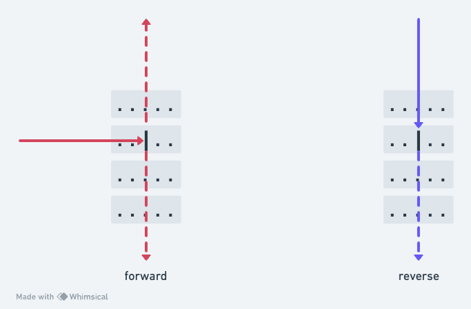
Part 2 of this problem involves shining a laser beam in from every possible entry point in the grid to see which one maximizes the number of energized squares the laser passes through. It parallelizes nicely so it was one of the days I’d optimized by splitting across cores, and had the longest single core runtime after the rest of my optimizations. Therefore I decided to take a closer look. I managed to get this runtime down to 0.35s on a single core from 0.9s on a single core. The trick here is to note that there are a whole bunch of grid entry points that can’t possibly contribute a greater number of energized cells than ones we’ve already tested and avoid simulating them at all. Let me explain - here’s a grid with a couple of mirrors in it. When we shine the laser in from the left side on the second row, it will reflect from the first mirror, hit the second mirror, reflect again and exit the grid on row 4 on the right. If we now shine another beam in the opposite direction from the same spot the first one exited, it will follow the same path in reverse and exit where we shone the first beam in, lighting exactly the same number of cells in the grid.
If the grid consisted only of mirrors, everything would be perfectly symmetrical and it’s pretty clear that we don’t need to test entry points where we’ve already seen a beam exit as they will not increase the potential total number of energized cells.
At the end of my trybeam function, anywhere the laser exits the grid, I capture the exit cell:
    def trybeam(ix, iy, idx, idy):
        ...
        exits = set()
        while beams:
            ...
            # if we're still on the grid
            if 0 <= x < w and 0 <= y < h:
                # do stuff
            else:
                exits.add((x, y))
        return len(energize), exits
And in part 2, rather than fire the laser in from every edge square, I first check to see if a beam exited there and skip it if we saw one already, plus add any new exits to the set we will skip in future.
    ...
    for y in range(h):
        if (-1, y) not in exits:
            mi, exits_ = trybeam(0, y, 1, 0)
            mm = max(mm, mi)
            exits.update(exits_)
    ...
Whoah, whoah, whoah, I hear you say - not so fast! That’s all well and good for mirrors which are symmetrical, but what about those splitters!?
Well, it turns out they have a pretty interesting property.
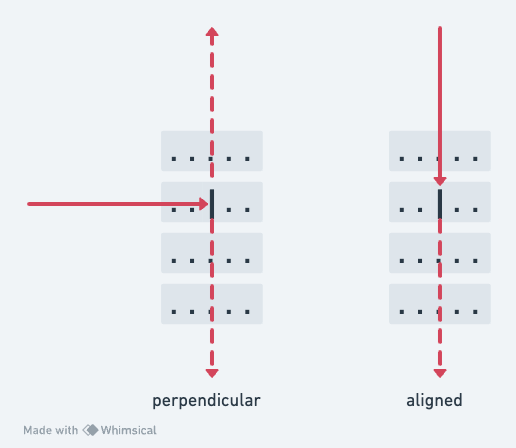
Here’s a grid with a splitter - if we fire the laser in perpendicular to the splitter, it will emit two beams at right angles:
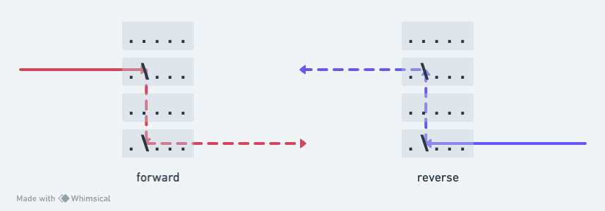
But, if you pass the laser parallel to the splitter, it continues straight on. So if we take either of the exits of that first beam and fire the laser back in, it continues on to hit the same squares the “other” half hit, but does not pop out sideways to light the squares that the original laser energized before hitting the splitter:
So, for a beam that has gone through a splitter, passing it back (from either side) in the opposite direction can light fewer cells (strictly, fewer or the same number) than going in the perpendicular direction, so when we’re looking to find a maximum number we can safely skip these paths too!
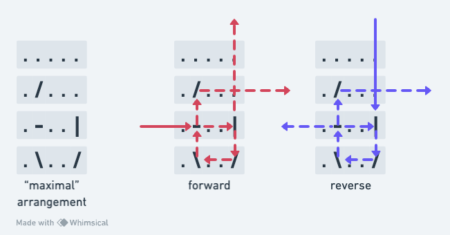 The “maximal” case where splitter return paths light the same number of squares due to strategic placement of mirrors to wrap the beam back around to perpendicular for each case.
This trick is a ~3x speedup - you can find the full solution here.
A few other themes
1D “grids” can be faster than 2D
azzal07 worked on and improved my solution to day 17 by using a fixed sized list for the bucket queue and switching to a one dimensional structure for the grid instead of a 2D array. This turns out to be a quite generalizable trick - I was also able to speed up my day 14 solution by switching to a 1D array.
With a 1D grid, parsing the input becomes:
D = [i.strip() for i in open("input", "r").readlines()]

g = list("".join(D))
w = len(D[0])
h = len(D)
and accessing a cell is g[y*w + x] instead of g[y][x] - this, somewhat surprisingly, yields a 10-20% speed up for problems where the grid is accessed a lot.
Don’t do work you don’t have to
This might sound like an insight from the dept of the bleedingly obvious, but it was striking to me how many places I could have the solution do less work if I really stared at it. Many of these cases involved rewriting code to be less elegant and simple. In that regard, the mentality you need to take when optimizing runtime is quite different from the best tactics for writing a good solution quickly during the live competition. A competition-time maxim I picked up from mcpower is write less code. The best/fastest competitors all have short solutions - less code equals fewer bugs. I had some elegantly short competition time solutions and to make them run faster had to get comfortable with losing that elegance. The best examples are day 22 and day 14. Day 22 involves dropping tetris-like blocks, then removing individual blocks from the resulting pile and seeing if others fall as a result. My original solution reused the code I wrote to drop bricks to see if any would move, less code, fewer bugs - this was a smart choice during the live competition. But a much faster algorithm is to note which blocks support each other during the first “drop” pass, then transitively navigate that structure when determining how many blocks will move when each one is exploded. This was a 40% speed up. Here’s the full solution.
Similarly, day 14 involves rolling stones on a grid northward, westward, southward and eastward a billion times and determining where they all end up (the crux of this solution is to figure out that the positions eventually start looping). I wrote this cute solution during the competition which only knew how to roll stones northward, then rotated the underlying grid to achieve the other directions. Less code, fewer bugs!
def roll_north(g,w,h):
    new_grid = [r[:] for r in g]
    for j in range(h):
        for i in range(w):
            if g[j][i] == "O":
                jj = j
                while jj >0 and not (new_grid[jj-1][i] == 'O' or new_grid[jj-1][i] == '#'):
                    jj -= 1
                new_grid[j][i] = "."
                new_grid[jj][i] = "O"
    return new_grid

def rotate_clock(g):
    return [list(x) for x in list(zip(*g[::-1]))]
...
for i in range(1000000000):
    for _ in range(4):
        g = roll_north(g,w,h)
        g = rotate_clock(g)
This was pretty fast, but not optimal rotate_clock makes a copy of the grid every time. The solution? Don’t copy the grid and write separate functions for roll_{north,west,south,east}. That, plus the 1D grid translates to a nearly 2x speedup (code).
Conclusion
This latest round of optimization was, again, a tremendous learning experience. For fun, I also put all the new solutions back into my (hideous) combined allatonce.py file, which runs all 25 days in parallel across multiple cores. This is now able to solve all of Advent of Code 2023 in just 0.48 seconds.
🚀 pypy3 allatonce.py
day06 0.0004s
...
day23 0.4632s
**** total time (s): 0.485254